Period life expectancy in Germany
Death counts in Germany between 2019 and 2020
In the light of the COVID-19 pandemic, researchers and journalists were highly interested in comparing the observed number of deaths in 2020 with annual death counts from previous years. Further, there is a still ongoing discussion about the impact of COVID-19 on life expectancy (LE). The relationship between increases/decreases in the annual death count observed in a year and changes in LE is not as clear as often suggested. In the following, I would like to share my analysis on the age distribution of deaths in 2019 and 2020, hoping to create some clarification. The calculations are based on mortality data for women and men in Germany downloaded from Desatis.
library(openxlsx)
setwd("d:/Rcode/Data")

###Data is available at www.destatis.de
Deaths.m <- read.xlsx("Sterbefälle.xlsx", sheet="Men")
Deaths.f <- read.xlsx("Sterbefälle.xlsx", sheet="Women")

Dx.2019.m <- Deaths.m$Deaths2019
Dx.2020.m <- Deaths.m$Deaths2020

Dx.2019.f <- Deaths.f$Deaths2019
Dx.2020.f <- Deaths.f$Deaths2020

rbind(
    cbind(X2019=sum(Dx.2019.m),
      X2020=sum(Dx.2020.m),
      Diff=sum(Dx.2019.m)-sum(Dx.2020.m)
      ),

    cbind(X2019=sum(Dx.2019.f),
      X2020=sum(Dx.2020.f),
      Diff=sum(Dx.2019.f)-sum(Dx.2020.f)
      )
)
## X2019 X2020 Diff
## [1,] 465885 492797 -26912
## [2,] 473635 492775 -19140The output shown above gives the total death count for men (first row) and women (second row) in 2019 and 2020. The difference between the two years is presented in the last column of the table. We observe more deaths in 2020 compared to 2019 for both genders. We know from previous analyses that excess deaths were not equally distributed over time and across regions. For example, the number of deaths was particularly high at the end of 2020. Analyzing these differences is, however, beyond the scope of this post. Instead, I focus on the average and calculate the mean age at death (MAD), the mode (the age with the highest observed death count), and the median (the age at which 50 percent of the total number of deaths have occurred). Please let me know if you know a better way to derive mode and median (maybe with decimals) without getting too sophisticated (e.g., modeling and predicting counts).
age <- 0:100
MAD.2019.m <- (sum((age+0.5)*Dx.2019.m))/sum(Dx.2019.m)
MAD.2020.m <- (sum((age+0.5)*Dx.2020.m))/sum(Dx.2020.m)
Mode.2019.m <- age[which.max(Dx.2019.m)]
Mode.2020.m <- age[which.max(Dx.2020.m)]
Median.2019.m <- age[which(cumsum(Dx.2019.m)>=(sum(Dx.2019.m)/2))[1]]
Median.2020.m <- age[which(cumsum(Dx.2020.m)>=(sum(Dx.2020.m)/2))[1]]

MAD.2019.f <- (sum((age+0.5)*Dx.2019.f))/sum(Dx.2019.f)
MAD.2020.f <- (sum((age+0.5)*Dx.2020.f))/sum(Dx.2020.f)
Mode.2019.f <- age[which.max(Dx.2019.f)]
Mode.2020.f <- age[which.max(Dx.2020.f)]
Median.2019.f <- age[which(cumsum(Dx.2019.f)>=(sum(Dx.2019.f)/2))[1]]
Median.2020.f <- age[which(cumsum(Dx.2020.f)>=(sum(Dx.2020.f)/2))[1]]

rbind(
    cbind(MAD.2019=MAD.2019.m,
      MAD.2020=MAD.2020.m,
      Diff=MAD.2019.m-MAD.2020.m
      ),

    cbind(MAD.2019=MAD.2019.f,
      MAD.2020=MAD.2020.f,
      Diff=MAD.2019.f-MAD.2020.f
      )
)
## MAD.2019 MAD.2020 Diff
## [1,] 76.05939 76.47146 -0.4120715
## [2,] 81.92622 82.18910 -0.2628851The MAD increased for both, women and men between 2019 and 2020. Accordingly, the analysis suggest that more people have died in 2020 but most deaths have occurred at relatively old ages. It is correct that this kind of analysis does not take into account changes in the age structure. Germany is an aging population and more persons at older ages will necessarily lead to an increase in the observed death count. The following graph shows the observed distribution of death. The vertical lines indicate the MAD, the modal age at death, and the median.
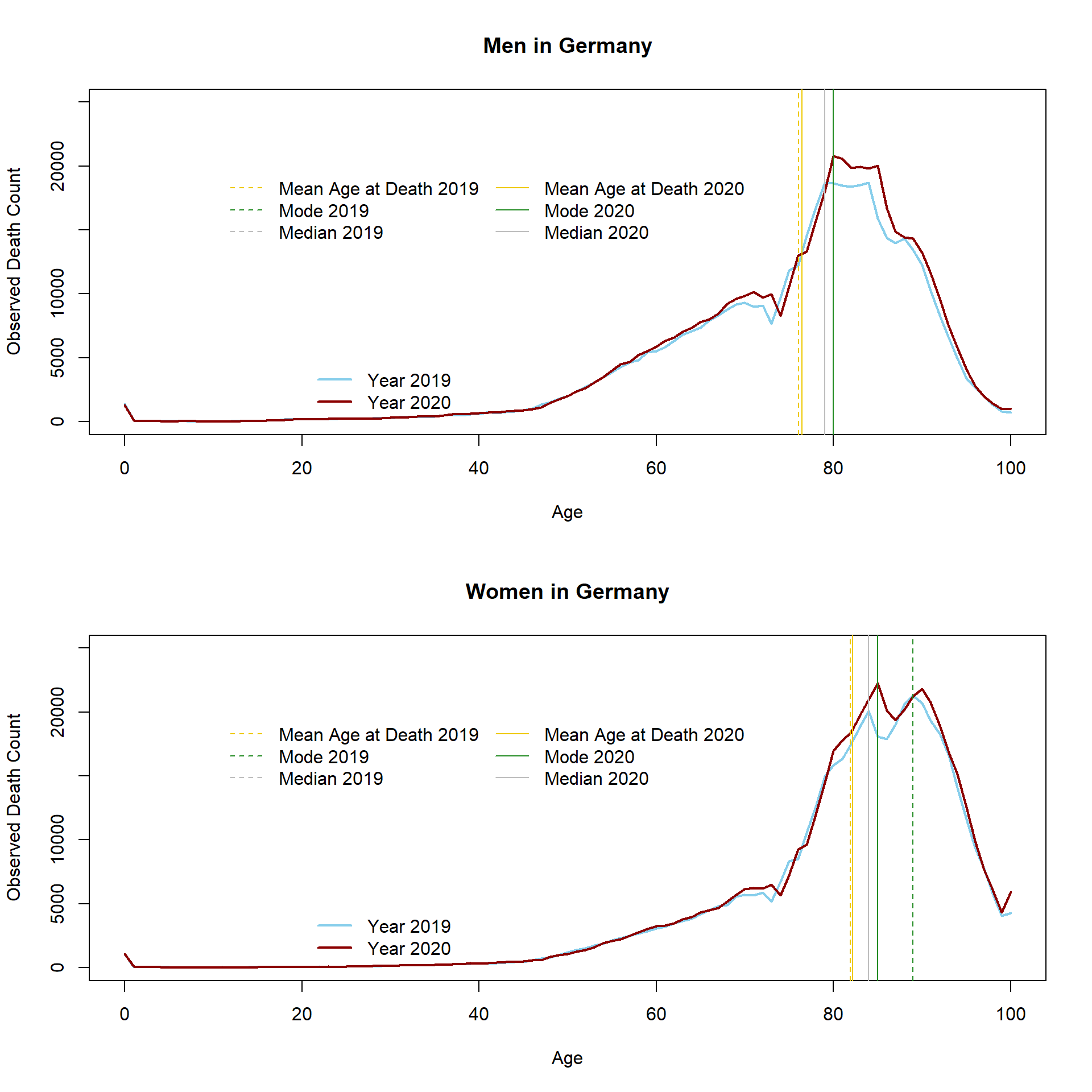 Especially at higher ages (between 80 and 90), more deaths have been observed in 2020 compared to the previous year. More information about the relationship between longevity and trends in the mean age at death, modal age at death, and median age at death can be found in Canudas-Romo (2010).
Standardized Mean Age at Death
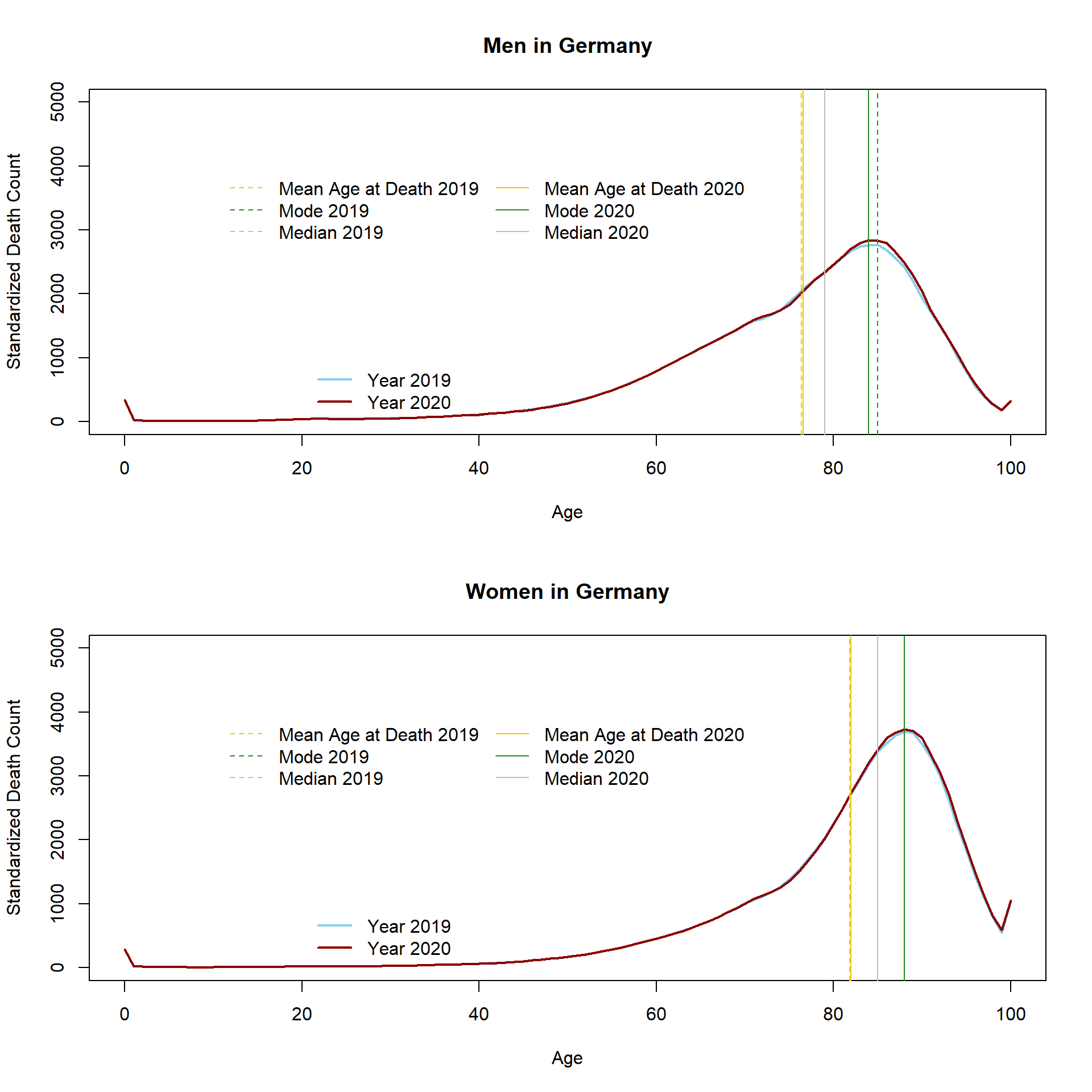
In the next step, I will calculate another MAD which is less common but, I believe, very interesting. It is the standardized MAD which has been described by Bongaarts and Feeney (2003). The standardized MAD is the mean age at death that would have been observed if the present population had experienced a constant inflow of births. In other words, the initial size of each birth cohort is constant or how Guillot (2006) put it “MAD can be interpreted as the population mean age at death at time t, controlling for changes in the initial size of cohorts.” I used the cohort life tables provided by Destatis in order to calculate the standardized number of deaths in 2019 and 2020. This allows obtaining standardized MAD, mode, and median values.
###Standardized death count calculated on the basis of cohort life tables provided at www.destatis.de
library(openxlsx)
setwd("d:/Rcode/Data")

Dx.standardized <- read.table("MAD_dx.txt")

Std.Dx.2019.m <- Dx.standardized$dx.2019[Dx.standardized$Sex=="M"]*100000
Std.Dx.2020.m <- Dx.standardized$dx.2020[Dx.standardized$Sex=="M"]*100000

Std.Dx.2019.f <- Dx.standardized$dx.2019[Dx.standardized$Sex=="F"]*100000
Std.Dx.2020.f <- Dx.standardized$dx.2020[Dx.standardized$Sex=="F"]*100000


age <- 0:100
Std.MAD.2019.m <- (sum((age+0.5)*Std.Dx.2019.m))/sum(Std.Dx.2019.m)
Std.MAD.2020.m <- (sum((age+0.5)*Std.Dx.2020.m))/sum(Std.Dx.2020.m)
Std.Mode.2019.m <- age[which.max(Std.Dx.2019.m)]
Std.Mode.2020.m <- age[which.max(Std.Dx.2020.m)]
Std.Median.2019.m <- age[which(cumsum(Std.Dx.2019.m)>=(sum(Std.Dx.2019.m)/2))[1]]
Std.Median.2020.m <- age[which(cumsum(Std.Dx.2020.m)>=(sum(Std.Dx.2020.m)/2))[1]]

Std.MAD.2019.f <- (sum((age+0.5)*Std.Dx.2019.f))/sum(Std.Dx.2019.f)
Std.MAD.2020.f <- (sum((age+0.5)*Std.Dx.2020.f))/sum(Std.Dx.2020.f)
Std.Mode.2019.f <- age[which.max(Std.Dx.2019.f)]
Std.Mode.2020.f <- age[which.max(Std.Dx.2020.f)]
Std.Median.2019.f <- age[which(cumsum(Std.Dx.2019.f)>=(sum(Std.Dx.2019.f)/2))[1]]
Std.Median.2020.f <- age[which(cumsum(Std.Dx.2020.f)>=(sum(Std.Dx.2020.f)/2))[1]]

rbind(
    cbind(MAD.2019=Std.MAD.2019.m,
      MAD.2020=Std.MAD.2020.m,
      Diff=Std.MAD.2019.m-Std.MAD.2020.m
      ),

    cbind(MAD.2019=Std.MAD.2019.f,
      MAD.2020=Std.MAD.2020.f,
      Diff=Std.MAD.2019.f-Std.MAD.2020.f
      )
)
## MAD.2019 MAD.2020 Diff
## [1,] 76.37203 76.56336 -0.1913279
## [2,] 81.83031 81.96213 -0.1318239By definition, this measure is not affected by changes in the age structure. Also the standardized MAD increased between 2019 and 2020. The standardized distribution is smoother as compared to the unstandardized one, indicating that some of the bumps can be ascribed to differences in the size of birth cohorts.
Period life expectancy in 2019 and 2020
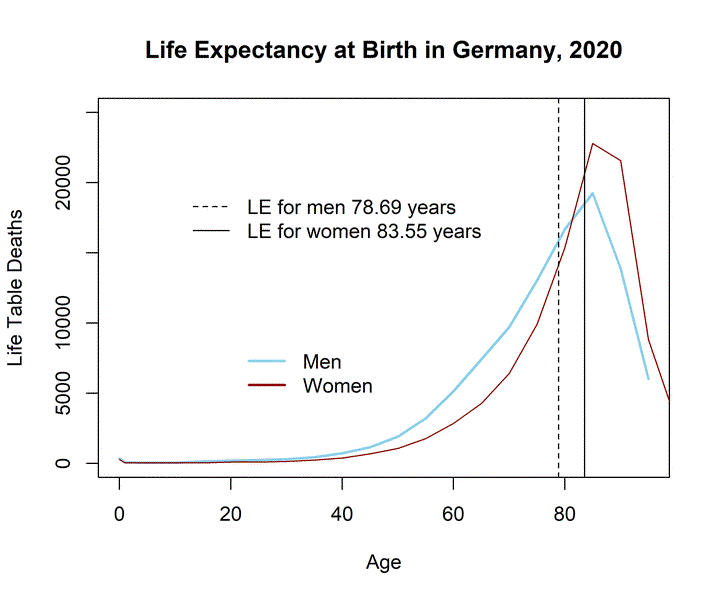
Last but not least, I provide estimates for the most prominent mortality indicator, i.e., period life expectancy at birth (LE). As a reminder, LE is the mean age at death for the period life table population. The life table population is derived from age-specific death rates which are again provided by Destatis. This is the exact link: https://www.destatis.de/DE/Presse/Pressemitteilungen/2021/07/PD21_331_12621.html. I simply copied the values from the table to my R session, e.g., “Germany.mx.2019.women <- c(…)” (code is omitted). Please note, the death rates refer to 5-years age intervals. For this reason, I calculated an abridged life table. The R package DemoTools" by Tim Riffe et al. (2019) helped me. Thanks! The LE values for 2019 and 2020 in Germany based on single-age specific period life tables will be published at www.lebenserwartung.info and differ slightly from the LE estimates presented in this post (the single-age specific life tables with an open age-interval at higher ages yield more precise LE estimates).
###Following the DemoTools documentation example, the abridged life table is constructed as:
library(DemoTools)
## Lade nötiges Paket: RcppAge <- c(0, 1, seq(5, 95, by = 5))
AgeInt <- age2int(Age,OAvalue = 5)
LE.women.2019 <- lt_abridged(Age=Age, nMx = Germany.mx.2019.women/1000, sex = "female",
AgeInt = AgeInt, axmethod = "un", mod = FALSE, OAnew = 100, a0rule ="cd")
LE.women.2020 <- lt_abridged(Age=Age, nMx = Germany.mx.2020.women/1000, sex = "female",
AgeInt = AgeInt, axmethod = "un", mod = FALSE, OAnew = 100, a0rule ="cd")
LE.men.2019 <- lt_abridged(Age=Age, nMx = Germany.mx.2019.men/1000, sex = "male",
AgeInt = AgeInt, axmethod = "un", mod = FALSE, OAnew = 100, a0rule ="cd")
LE.men.2020 <- lt_abridged(Age=Age, nMx = Germany.mx.2020.men/1000, sex = "male",
AgeInt = AgeInt, axmethod = "un", mod = FALSE, OAnew = 100, a0rule ="cd")
###Compare LE estimates by age
###Men in Germany
round(cbind(Age=Age[c(1,15)],
LE.2019=LE.men.2019$ex[c(1,15)],
LE.2020=LE.men.2020$ex[c(1,15)],
Diff=LE.men.2019$ex[c(1,15)]-LE.men.2020$ex[c(1,15)]),2)## Age LE.2019 LE.2020 Diff
## [1,] 0 78.86 78.69 0.17
## [2,] 65 18.15 17.92 0.23###Women in Germany
round(cbind(Age=Age[c(1,15)],
LE.2019=LE.women.2019$ex[c(1,15)],
LE.2020=LE.women.2020$ex[c(1,15)],
Diff=LE.women.2019$ex[c(1,15)]-LE.women.2020$ex[c(1,15)]),2)## Age LE.2019 LE.2020 Diff
## [1,] 0 83.64 83.55 0.10
## [2,] 65 21.35 21.23 0.12###getting mode
Mode.LT.2019.f <- Age[which.max(LE.women.2019$ndx)]
Mode.LT.2020.f <- Age[which.max(LE.women.2020$ndx)]
Mode.LT.2019.m <- Age[which.max(LE.men.2019$ndx)]
Mode.LT.2020.m <- Age[which.max(LE.men.2020$ndx)]As presented in the table above, LE slightly decreased for both genders. The distribution of life table deaths is plotted below. It shows the age-specific number of deaths for the life table cohort which has been exposed to the age-specific mortality rates observed in Germany.
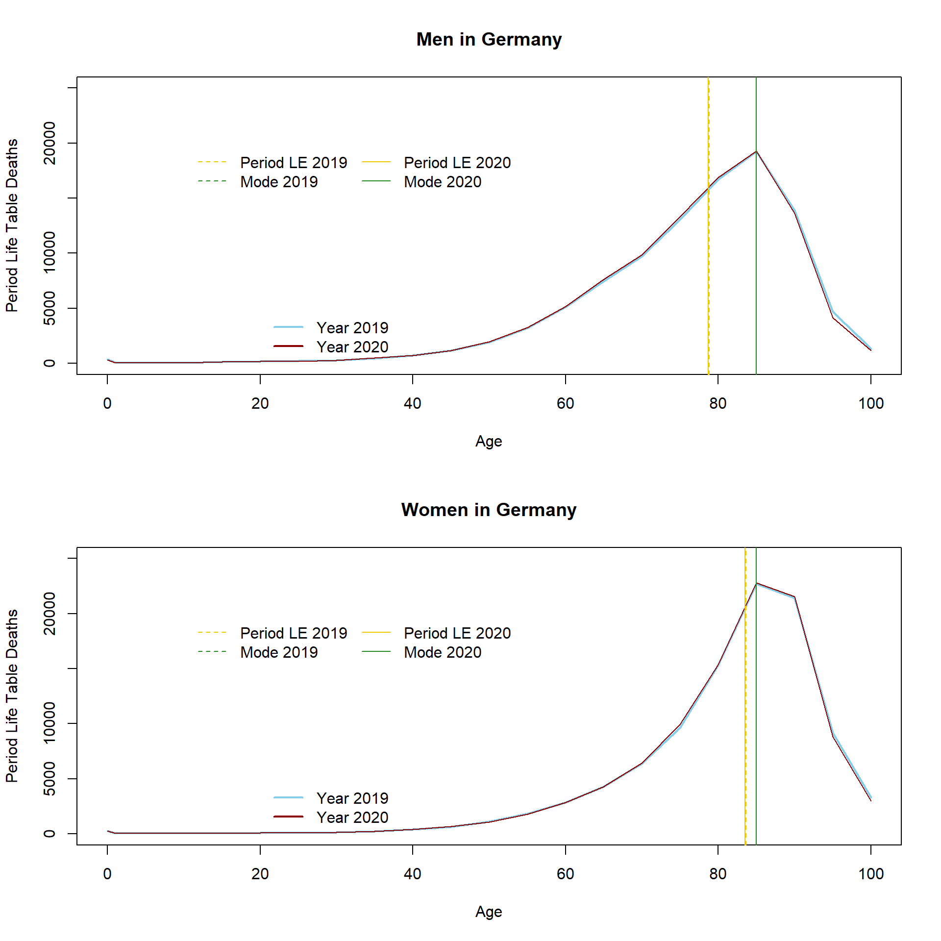 This time I do not calculate the median because, as already mentioned, data was only available in 5-years age intervals. The median should lay somewhere in the age interval 80-84 for men and 85-89 for women. The MAD (or LE) in the period life table population is higher compared to the the unstandardized and standardized MAD. Another way to look at LE is imagining Germany would be trapped in a loop where it repeats the year 2020 over and over again for about 100 years (I know, nobody wants this). A lucky child who is born at the beginning of this loop can expect to live 83.55 years in case it´s a girl and 78.69 years if it´s a boy. Obviously, this scenario is unlikely and LE is usually not a good estimate for the expected life time of any actual group of individuals (Goldstein and Wachter 2006). It is rather a convenient way to summarize period death rates and examine period shocks in health and mortality. The increase in the observed death rates for the elderly in 2020 is reflected by the decrease in period LE in 2020. Yet, the indicator is not free of limitations and can lead to misleading conclusions regarding levels and trends in population health (Luy et al. 2020; Modig, Rau, and Ahlbom 2020; Heuveline 2021). In comparison to other countries, Germany`s LE reduction is small. It is important to note that changes in death rates at different ages will affect LE differently (Vaupel 1986). It is therefore not so easy to translate increases in death counts at any age directly into LE reductions. For instance, the reduction in LE is higher at age 65 compared to LE at birth, indicating that death rates have mostly increased at older ages. The largest increase in mortality is observed for older men (LE at age 65 decreased by 0.23 years between 2019 and 2020). For more information about differences in LE in Germany, including differences between genders, East and West Germany, socioeconomic groups, and regions, see Marc Luy´s webpage www.lebenserwartung.info and for more country-specific results see the work by Aburto et al. (2021), which also features an interactive dashboard.
References
Canudas-Romo, V. (2010). Three Measures of Longevity: Time Trends and Record Values. Demography 47(2):299–312.
Bongaarts, J. and Feeney, G. (2003). Estimating mean lifetime. PNAS 100(23):13127-13133.
Guillot, M. (2006). Tempo effects in mortality: An appraisal. Demographic Research 41(1):1-26.
Riffe, T., Aburto, J.M., Alexander, M., Fennell, S., Kashnitsky, I., Pascariu, M., Gerland, P. (2019). DemoTools: An R package of tools for aggregate demographic analysis. github.com/timriffe/DemoTools.
Goldstein, J., & Wachter, K. (2006). Relationships between Period and Cohort Life Expectancy: Gaps and Lags. Population Studies 60(3):257-269.
Luy, M., Di Giulio, P., Di Lego, V., Lazarevič, P., Sauerberg, M. (2020). Life Expectancy: Frequently Used, but Hardly Understood. Gerontology 66:95-104.
Modig, K., Rau, R., Ahlbom, A. (2020). Life expectancy: what does it measure? BMJ Open 10(7):e035932.
Heuveline, P. (2021). The Mean Unfulfilled Lifespan (MUL): A new indicator of the impact of mortality shocks on the individual lifespan, with application to mortality reversals induced by COVID-19. PLoS ONE 16(7):e0254925.
Vaupel, J. (1986). How changes in age-specific mortality affects life expectancy. Population Studies 40:147-157.
Aburto, J.M., Schöley, J., Zhang, L., Kashnitsky, I., Rahal, C., Missov, T.I., Mills, M.C., Dowd, J.B., Kashyap, R. (2021). Recent Gains in Life Expectancy Reversed by the COVID-19 Pandemic. Medrxiv Link.